Photogrammetry plays a crucial role in capturing and processing spatial information. The technology allows us to calculate highly accurate 3D models and coordinates from photographs and imagery. This requires that the camera used be calibrated. This article describes how a camera calibration works.
The article on the camera model described how a camera is mathematically modeled. This modeling can then be used to calculate coordinates using triangulation and bundle block adjustment. This article describes how the elements from the mathematical modeling of the camera can be determined using a camera calibration.
Focal length
In the observation equations we find parameters for the terrain coordinates of the tie points and for the external orientation of the picture. All these parameters are included as unknown parameters in the adjustment. However, in the observation equation we also encounter 𝑓, the focal length.
In many projects in aerial photogrammetry, we do not have to worry about this value. The camera manufacturer provides an annual calibration report that includes the correct value for 𝑓. In close-range applications, or when using a drone, we usually do not know the focal length. It must be determined by calibration.
From a bundle block adjustment perspective, fortunately, calibrating a focal length is straightforward. We can easily enter 𝑓 as an unknown parameter and estimate a value for the focal length in the adjustment. This does impose additional requirements on the survey, as the probability of a singular matrix is higher in this case. For example, in the case of drone and aerial photogrammetry, focal length and flight altitude are highly correlated. This can be overcome by including surveys from two different flight altitudes in one adjustment.
Principal point offset
It follows from the central projection that the origin of the photographic system lies at the center of projection. Therefore, the center of a photo has coordinates (0,0,-𝑓). This is also how it was defined in the pinhole camera model in the camera model article. However, the reality is that the center of the sensor is rarely exactly below the projection center. Due to inaccuracies during the manufacturing of the camera or objective lens, the sensor is usually slightly offset.
A light ray incident perpendicular to the sensor plane has coordinates slightly off-center at that point. This point, defined by the line that goes perpendicular to the sensor plane and passes through the projection center, is called the principal point. The distance between the center of the sensor and the principal point is called the principal point offset. Until now, all equations assumed that the principal point offset was equal to 0. Now that this turns out not to be the case, the equations must be adjusted accordingly. The adjusted collinearity equations are:
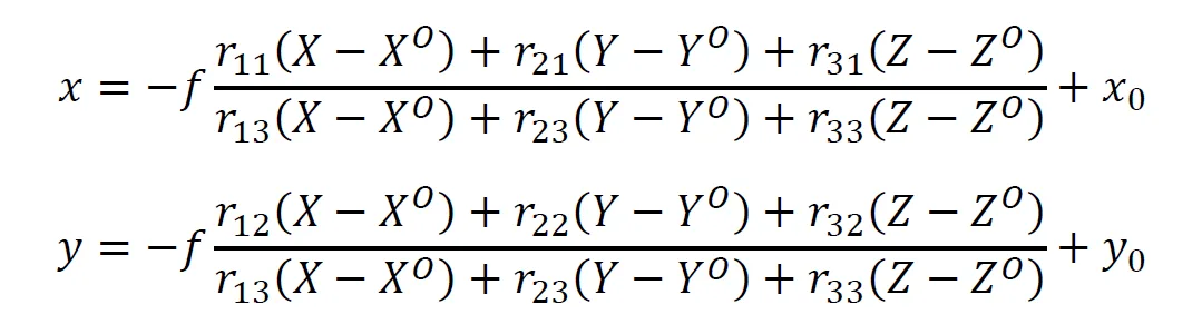
In this, 𝑥0 and 𝑦0 represent the principal point offset (Figure 1). Again, the principal point offset can be found in the camera calibration report from the supplier of a photogrammetric camera. For close-range applications, the value should be determined by including the principal point offset as an unknown in the adjustment.
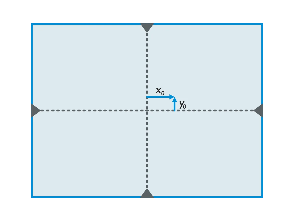
Figure 1 - Principal point on a sensor
Lens distortion
The assumption that light rays pass through the pinhole camera hole along a straight line does also not hold true. This is because there is not a hole, but an objective lens is in place. Even with high-quality objective lenses, there will be some degree of distortion, making the assumption that light rays go straight through no longer true. Therefore, lens distortion must be determined.
Lens distortion is divided into two components: radial lens distortion and tangential lens distortion. The radial lens distortion is described by a polynomial. For each distance from the principal point, this polynomial gives the correction to be applied. Usually Brown's lens distortion model is used for the polynomial. Other forms of distortion can also be modeled, such as decentering and skewing.
Additional parameters
The description of principal point offset and lens distortion shows that it is possible to apply various corrections to photo coordinates. The magnitude of these corrections can be estimated in the bundle block adjustment. Many photogrammetric software programs have the option for additional parameters. These are additional unknowns that can be added to model other deviations from the standard collinearity equation. There are additional parameters with (historical) importance. For example, many software programs have additional parameters to apply a bias resulting from scanning analog photographs. Some examples of additional parameters found in bundle block adjustment software include:
- Distortions due to scanning;
- Distortions due to warping of analog photos;
- Affine transformation;
- Distance between the GNSS/INS system and the projection center of the camera (the lever arms);
- Rotation between the GNSS/INS system and photo system (the misalignment);
- Correction for cycle slip per flight strip (an incorrectly resolved phase ambiguity in the GNSS calculation);
- Correction for rolling shutter effects;
- Constant shift of the projection center.
Additional parameters may be added to a bundle block adjustment only if they are physically justifiable. Thus, the application of the additional parameters must be explainable from the conditions during recording.
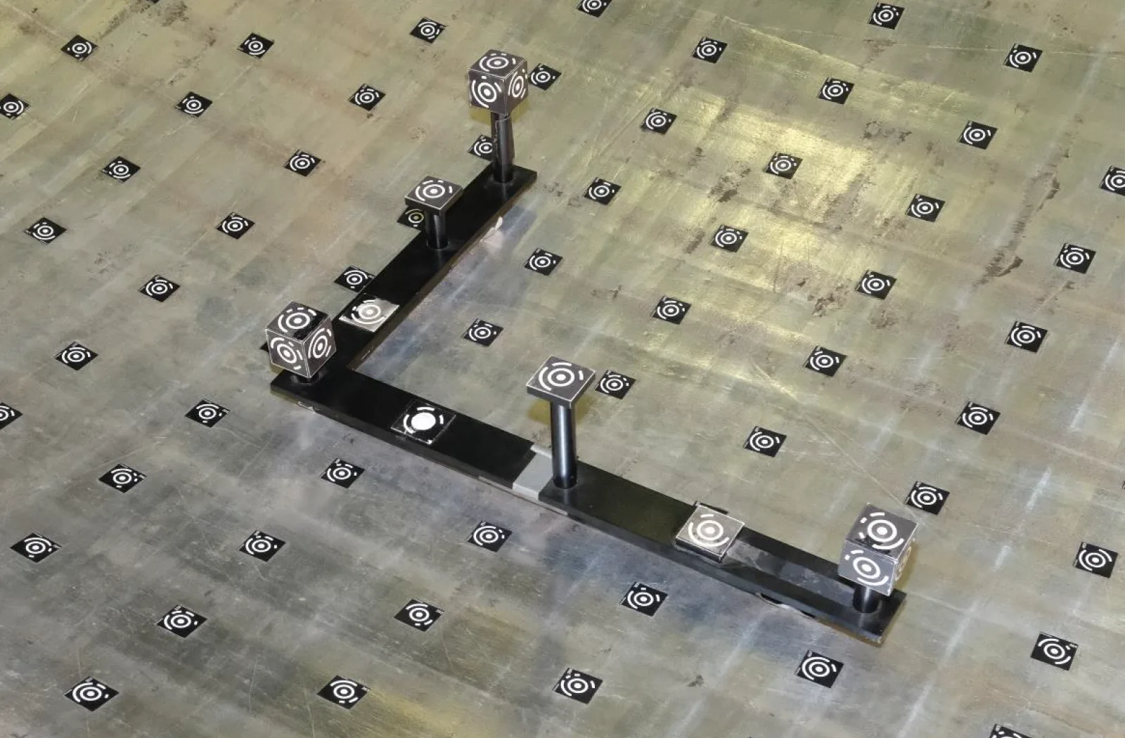
Laboratory Calibration
The above shows that it is possible to perform a camera calibration while recording. Nevertheless, the best results can be expected in a calibration in a controlled environment. A so-called laboratory calibration. Geodelta has the facilities it for performing a laboratory calibration and can also support in performing calibrations during a special calibration survey flight.